The Key Points
We introduce our first multi-variate feature extraction problem, the problem of learning with side information. Here, we wish to extract a $k$-dimensional feature of the data $\mathsf x$ that carries useful information to infer the value of the label $\mathsf y$, while excluding the information that a jointly distributed side information $\mathsf s$ can provide. We use this example to develop the underlying geometric structure of multi-variate dependence, and demonstrate how to use the nested H-Score networks to make projections according to these structures to get good solutions.
Previously
We started by observing that the dependence between two random variables $\mathsf x$ and $\mathsf y$ can be decomposed into a number of modes, each mode as a simple correlation between a feature $f_i(\mathsf x)$ and a feature $g_i(\mathsf y)$. We formulated the modal decomposition as the optimization problem
\[\begin{equation}
(f^\ast_{[k]}, g^\ast_{[k]}) =\arg\min_{(f_1, \ldots f_k \in \mathcal {F_X}, g_1, \ldots g_k \in \mathcal {F_Y})} \; \left\Vert \mathrm{PMI}- \left(\sum_{i=1}^k f_i \otimes g_i\right)\right\Vert^2
\end{equation}\]
with the constraints that both $f^\ast_1, \ldots, f^\ast_k$ and $g^\ast_1, \ldots, g^\ast_k$ are collections of orthogonal feature functions; and that the correlation $\sigma_i = \rho(f^\ast_i(\mathsf x), g^\ast_i(\mathsf y))$ are arranged in a descending order.
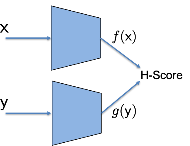
We proposed the H-Score networks as a numerical approach, using interconnected neural networks to learn the modal decomposition from data. For two collections of feature functions $f_{[k]}\subset \mathcal {F_X}, g_{[k]} \subset \mathcal {F_Y}$, written in vector form as $\underline{f}, \underline{g}$, the H-score is defined as
\[H(\underline{f}, \underline{g}) =\mathrm{trace} (\mathrm{cov} (\underline{f}, \underline{g})) - \frac{1}{2} \mathrm{trace}(\mathbb E[\underline{f} \cdot \underline{f}^T] \cdot \mathbb E[\underline{g} \cdot \underline{g}^T])\]
 |
 |
| H-Score Network |
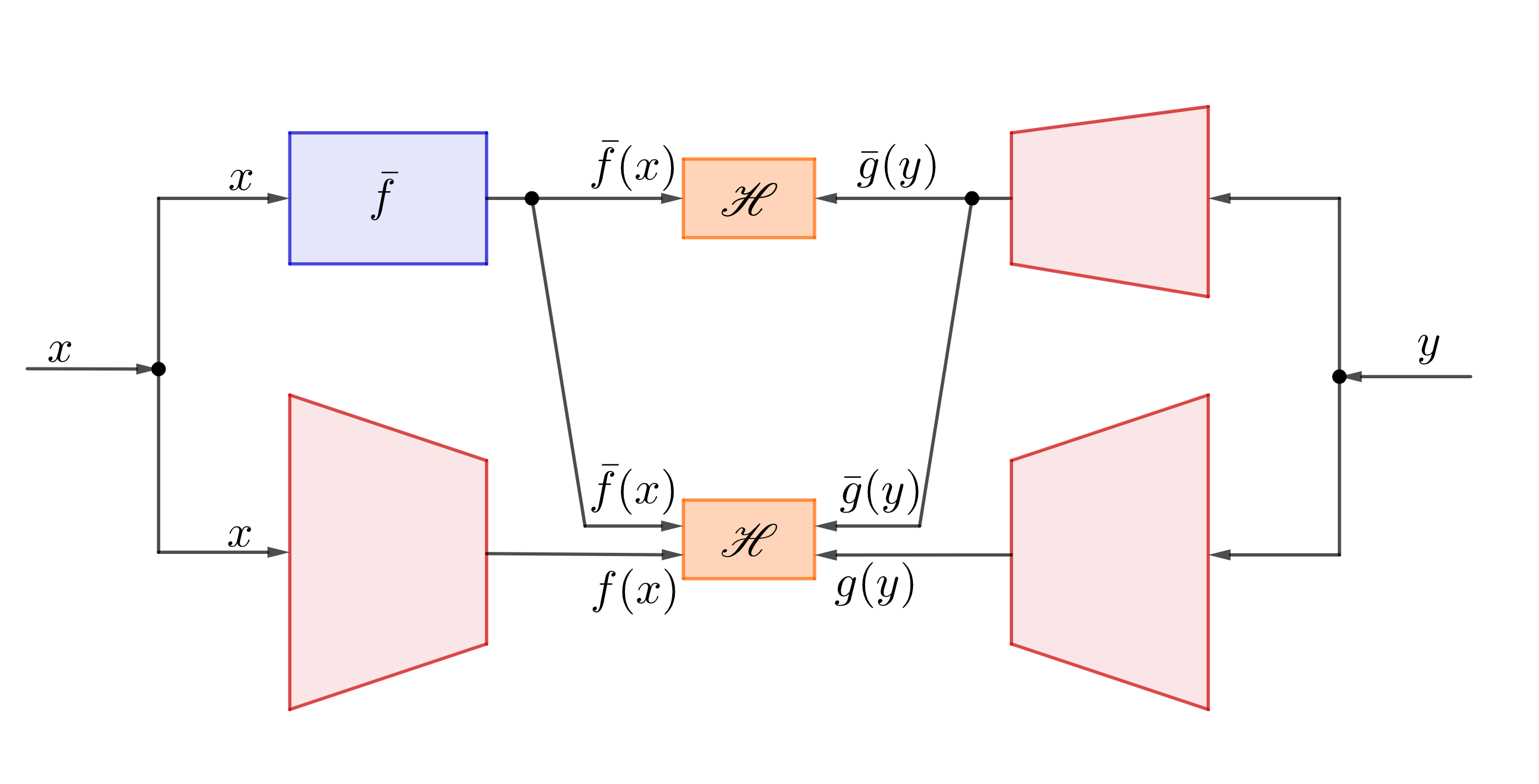
Nested H-Score Network to find features orthogonal to a given $\bar{f}$ |
We showed that maximizing the H-score is equivalent as solving the optimization problem in (1), only without some of the constraints. As a step to enrich our toolbox for extracting feature functions, we also developed the Nested H-Score networks to learn feature functions that are orthogonal to a given functional subspace. We give examples to demonstrate that such a projection operation in the functional space can be quite versatile, including enforcing all the desired constraints in the original modal decomposition problem (1).
These previous results now include the main tools we need to proceed: to find a limited number of information carrying feature functions and to make projections in functional space, which can all be learned directly from data using interconnected neural networks. In this page, we start to make the case that these are the critical building blocks for more complex multi-variate learning problems.
 |
| Feature Extraction with Side Information |
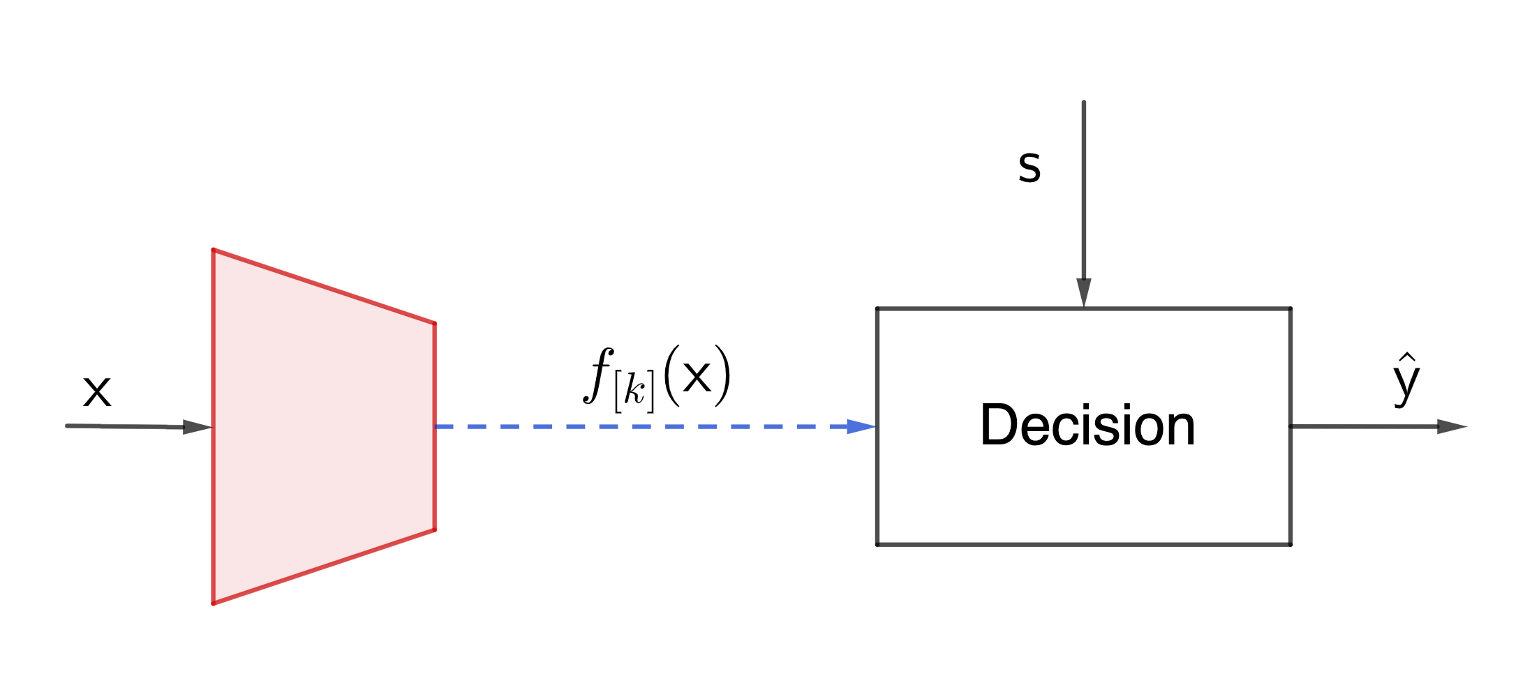
We consider the multi-variate learning problem as shown in the figure. Here, we assume that the data $\mathsf x$, the label $\mathsf y$, and the side information $\mathsf s$ are jointly distributed according to some model $P_{\mathsf {xys}}$ which is not known. Our goal is to find a $k$-dimensional feature function $f_{[k]} = [f_1, \ldots, f_k] : \mathcal X \to \mathbb R^k$, such that when we observe the value of $\mathsf x$, we can infer the value of $\mathsf y$ based on these $k$ features. The only difference between this and a conventional learning problem is that we assume the side information $\mathsf s$ can be observed at the decision maker. That is, our decision is based on the value of $\mathsf s$ and the features: $\widehat{\mathsf y} (f_{[k]}(x), s)$. More importantly, when we extract the feature functions, we know that such side information is available at the decision maker.
As a start point, we assume we have plenty of samples $(x_i, y_i, s_i), i=1, \ldots$ jointly sampled from the unknown model. Also we assume that the decision maker employs the optimal way to combine the side information $\mathsf s$ and the recieved $k$ features of $\mathsf x$ to estimate the value of $\mathsf y$. We can imagine a neural network is used to learn this decision function perfectly. The focus of this problem is how to find the $k$ feature functions to best facilitate this decision making.
The main tension of the problem is on having a limited number of $k$ features, which is often much lower dimensional representation of the data $\mathsf x$. Intuitively, we want the features to be about the dependence between $\mathsf x$ and $\mathsf y$, so that we can make good predictions; yet we would like to avoid reporting any information that the side information $\mathsf s$ can provide. Related problems can be found in the context of protecting sensitive information, fairness in machine learning, and many other multi-terminal information theory problems. The difficulty here is that we would like learn these feature functions using neural networks, and thus enjoy the computational efficiency and flexibility therein, but we have the additional task to tune the feature functions to avoid overlapping contents. It turns out what we need is a projection operation in the functional space.
Decomposition of Multi-Variate Dependence
For this problem, the dependence we would like to work on is the dependence between $\mathsf x$ and $(\mathsf {s,y})$. We write the PMI as
\[\mathrm{PMI}_{\mathsf {x; s,y}} = \log \frac{P_{\mathsf {xsy}}}{P_{\mathsf x}\cdot P_{\mathsf {sy}}} \; \in \mathcal {F_{X\times S\times Y}}\]
For this space of joint functions, we define inner product with reference distribution $R_{\mathsf {xsy}} = R_{\mathsf x}R_{\mathsf {sy}}$, parallel the definition of modal decomposition, with random variable $\mathsf y$ replaced by the tuple $\mathsf {(s,y)}$. We will take the local assumption that $P_\mathsf x \approx R_\mathsf x, P_{\mathsf {sy}} \approx R_{\mathsf {sy}}$. Under this assumption, in the following we do not distinguish between $\mathrm{PMI}_\mathsf{x;s,y}$ and its approximation
\[\widetilde{\mathrm{PMI}}_{\mathsf{x; s,y}} = \frac{P_\mathsf{xsy}}{P_\mathsf x\cdot P_{\mathsf {sy}}}-1.\]
Now we consider the subset of joint distributions that satisfy the Markov condition $\mathsf {x-s-y}$, which means that $\mathsf x$ is independent of $\mathsf y$ given $\mathsf s$. The corresponding PMI functions form a linear subspace. The linearity follows from the fact that conditional independence is a set of linear (equality) constraints on the joint distribution. We denote this subspace as $\mathcal M$.
For a general PMI function, we now decompose that into the component in $\mathcal M$ and that orthogonal to $\mathcal M$.
Definition: Markov Component and Conditional Dependence Components
For any given PMI function, $\mathrm{PMI}_{\mathsf {x; s,y}} $, the Markov component is
\[\pi_M \stackrel{\Delta}{=}\Pi_M(\mathrm{PMI}_{\mathsf{x; s,y}}) = \arg\min_{\pi \in \mathcal M}\; \left\Vert \mathrm{PMI}_{\mathsf{x; s,y}} - \pi\right\Vert^2\]
The optimization is overall all valid PMI functions $\pi$ in $\mathcal M$, i.e. with a corresponding joint distribution of $\mathsf{x, s, y}$ that satisfies the Markov constraint $\mathsf {x-s-y} $. The norm $\Vert\cdot \Vert$ in the objective function is defined on the functional space with reference distribution $R_{\mathsf {xsy}} = P_{\mathsf x}P_{\mathsf{sy}}$.
The Conditional Dependence Component is
\[\pi_C \stackrel{\Delta}{=}\mathrm{PMI}_{\mathsf{x; s,y}} - \pi_M\]
By definition, $\pi_C$ is the error of a linear projection, so we have $\pi_C \perp \mathcal M$, and the Pythagorean relation
\[\Vert \mathrm{PMI}_{\mathsf{x; s,y}}\Vert^2 = \Vert \pi_M\Vert^2 + \Vert \pi_C\Vert^2\]
As we stated in the properties of modal decomposition, under the local assumption, we have $\Vert \mathrm{PMI}_{\mathsf {x; s,y}}\Vert^2 \approx 2\cdot I(\mathsf x; \mathsf {s,y})$. Here one can show an additional fact that $\Vert \pi_M\Vert^2 \approx 2 \cdot I(\mathsf x; \mathsf s)$. From that, we also have $\Vert \pi_c \Vert^2 \approx 2 \cdot I(\mathsf x; \mathsf y \vert \mathsf s)$. Thus, the above Pythagorean relation is simply a geometric version of the chain rule of mutual information. It decomposes the dependence between $\mathsf x$ and a pair of random variables $\mathsf {s,y}$ into two orthogonal components: one follows the Markov constraint and only captures the $\mathsf {x-s}$ dependence, and the other is the conditional dependence between $\mathsf x$ and $\mathsf y$ conditioned on $\mathsf s$.
Going back to our problem of learning with side-information. It is clear at this point that in extracting the features of $\mathsf x$, we do not want any component in $\mathcal M$, since that is only helpful to predict the value of $\mathsf s$, which is already available at the decision maker.
The optimal choice of feature functions under this setup should be the $k$ strongest modes of $\pi_C$! By definition, we need to find the component of the PMI that is orthogonal to $\mathcal M$, which requires a projection operation in the functional space, and we can do that with a nested H-Score network.
Solution by Nested H-Score Networks
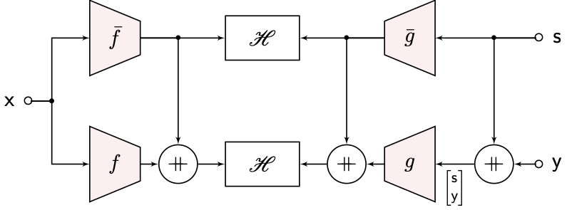 |
| Nested H-Score Network for Learning with Side Information |
The figure shows a solution to use nested H-Score networks to learn the modal decomposition of the $\pi_C$ component. Again, it is easier to see how it works with sequential training. We can first train the $\bar{f}, \bar{g}$ functions using the top H-score, which gives a modal decomposition of the $\mathsf {x-s}$ dependence, or equivalently, the $\pi_M$ component. Then we can freeze these choices of $\bar{f}, \bar{g}$, and train $f, g$ with the lower H-score, which gives the modal decomposition of the $\mathsf {x-(s,y)}$ dependence that is orthogonal to $\mathrm{span}(\bar{f} \otimes \bar{g})$, i.e., the span of all $\bar{f}_i \otimes \bar{g}_i$, $i = 1, \dots, \bar{k}$, which is aligned with the $\pi_C$ component that we want to find. Of course in practice, we train all networks simultaneously, and get the same desired result.
A slightly subtle point here is that in order to make the learned $f, g$ feature functions to be orthogonal to $\mathcal{M}$, we need to make sure that $\mathrm{span}(\bar{f} \otimes \bar{g})$ is large enough to cover $\mathcal M$. In particular, the dimensionality, i.e.,$\bar{k}$ the number of nodes at the output layer of the $\bar{f}$ and $\bar{g}$ networks, need to be large enough. More precisely, we will need $\bar{k} \geq \mathrm{rank} (P_{\mathsf {xs}})$. This is feasible particularly if the side information $\mathsf s$ is a small categorical variable. In such “nice” cases, we can show that the learned $f, g$ feature functions, with expressive neural networks and sufficient amount of training, are the desired modal decomposition of the $\pi_C$ component and hence are the optimal choice of features for the side information problem. A proof of this can be found in this paper.
In the case that we cannot guarantee that $\bar{k}$ is “large enough”, the situation is a bit more complex. Optimizing the top H-Score would fix $\bar{f}, \bar{g}$ on a $\bar{k}$ dimensional subspace of $\mathcal M$, and the nested structure guarantees that $f, g$ are trained to be orthogonal to this subspace, instead of $\mathcal M$, and thus can have components in $\mathcal M$. In the context of learning with side-information, this means that the extracted features would have some reduced level of repetitive information of the side information $\mathsf s$, but not completely repetition free.
Pytorch Implementation
Here is a colab demo of pytorch implementation, which also illustrates how to explore the dependence among multiple data observations using this nested H-score.
Going Forward
The important message here is that multi-variate dependence, represented in the functional space, can be decomposed into a number of subspaces, each corresponding to the dependence of a subset of the variables. Thus, in problems with more than two random variables involved, such as distributed learning, learning with time-varying models, with multiple tasks, with sensitive information, etc., we often need to separate the observed information according to these subspaces, and treat different parts of the information differently. Nested H-Score networks are a good method for this task of separating different types of information, by making projections in the functional space, without changing the objective function or brute-force post processing that is separated from the training process. We view this as an attestation of the power of the geometric view of the statistical dependence and the algorithms based on such insights. We will post some more examples in the same spirit, where the information geometric view can lead to some unconventional ways to use neural networks.