The Key Points
H-score is our first step introducing neural network based methods to compute modal decomposition from data. It is a loss metric used in the training of neural networks in a specific configuration. The result is approximately equivalent as a conventional end-to-end neural network with cross entropy loss, with the additional benefit of allowing direct controls of the chosen feature functions. This can be useful in applications with known structures or constraints of feature functions. Conceptually, the use of H-score networks turns the design focus onto functional operations, and serves as a stepping stone for the solutions to more complex problems.
The H-score Network
The motivation of modal decomposition is to find the rank-$k$ approximation
\[\begin{equation}
(f^\ast_1, g^\ast_1), \ldots, (f^\ast_k, g^\ast_k) =\arg\min_{(f_1, \ldots f_k \in \mathcal {F_X}, g_1, \ldots g_k \in \mathcal {F_Y})} \; \left\Vert \mathrm{PMI}- \left(\sum_{i=1}^k f_i \otimes g_i\right)\right\Vert^2
\end{equation}\]
The above problem is slightly different from our original definition of modal decomposition, where we had a sequential way to find the $k$ modes. This procedure ensures the solution to satisfy a number of constraints: 1) the feature functions all have zero mean and unit variance; 2) the scaling factor of the $i^{th}$ mode, $\sigma_i$, is separated from the normalized features; 3) the feature functions are orthogonal: $\mathbb E[f^\ast_i f^\ast_j] = \mathbb E[g^\ast_i g^\ast_j] = \delta_{ij}$, and 4)there is a descending order of the correlation between $f^\ast_i$ and $g^\ast_i$. Equation (1) is thus different from the modal decomposition. One can either view this optimization to have all the above constraints written in the footnotes and thus be consistent with the modal decomposition, or we could think this in a loose sense as the low rank approximation of the PMI function with no constraints. When we design algorithms to compute the modal decomposition, sometimes only a subset of the above constraints are enforced. We will have a detailed discussion on how these changes affect the solutions later in this page.
For convenience we introduce a vector notation: we write column vectors $\underline{f} = [f_1(\mathsf x), \ldots, f_k(\mathsf x)]^T$, $\underline{g} = [g_1(\mathsf y), \ldots, g_k(\mathsf y)]^T$. Now under the local approximation, we replace $\mathrm{PMI}$ by
\[\widetilde{\mathrm{PMI}} = \frac{P_{\mathsf{xy}}- P_{\mathsf x} P_{\mathsf y}}{P_{\mathsf x}P_{\mathsf y}}\]
and compute the norm with respect to $R_{\mathsf {xy}} = P_\mathsf xP_\mathsf y$. This reduces the problem as
\[\begin{align*}
(\underline{f}^\ast, \underline{g}^\ast) =&\arg\max_{\underline{f}, \underline{g}} \; \sum_{i=1}^k \mathbb E_{\mathsf {x,y} \sim P_{\mathsf {xy}}}\left[ f_i(\mathsf x) g_i(\mathsf y)\right] - \mathbb E_{\mathsf x\sim P_\mathsf x}[f_i(\mathsf x)]\cdot \mathbb E_{\mathsf y\sim P_{\mathsf y}}[g_i(\mathsf y)]\\
&\qquad \qquad -\frac{1}{2} \sum_{i=1}^k\sum_{j=1}^k \mathbb E_{\mathsf x\sim P_{\mathsf x}}[f_i(\mathsf x)f_j(\mathsf x)] \cdot \mathbb E_{\mathsf y\sim P_\mathsf y}[g_i(\mathsf y)g_j(\mathsf y)]
\end{align*}\]
with a few steps of algebra hidden in here
$$
\begin{align*}
\zeta_1^k(P_{\mathsf {xy}}) &= \arg\min \; \left\Vert \widetilde{\mathrm{PMI}}- \left(\sum_{i=1}^k f_i \otimes g_i\right)\right\Vert^2\\
&= \arg \min \; \left\Vert \widetilde{\mathrm{PMI}} \right\Vert^2 - 2 \left\langle \widetilde{\mathrm{PMI}}, \left(\sum_{i=1}^k f_i \otimes g_i\right)\right\rangle + \left\Vert \left(\sum_{i=1}^k f_i \otimes g_i\right)\right\Vert^2\\
&= \arg\max \; \left\langle \widetilde{\mathrm{PMI}}, \left(\sum_{i=1}^k f_i \otimes g_i\right)\right\rangle -\frac{1}{2} \left\Vert \left(\sum_{i=1}^k f_i \otimes g_i\right)\right\Vert^2\\
&= \arg\max \; \sum_{x,y} P_{\mathsf x}(x) P_{\mathsf y}(y) \cdot \frac{P_{\mathsf {xy}} - P_{\mathsf x}P_{\mathsf y}(y)}{P_{\mathsf x}(x)P_{\mathsf y}(y)}\cdot \left(\sum_{i=1}^k f_i \otimes g_i\right)\\
&\qquad \qquad - \frac{1}{2}\cdot \sum_{xy} P_{\mathsf x}(x) P_{\mathsf y}(y) \cdot \left(\sum_{i=1}^k f_i \otimes g_i\right)^2\\
&= \arg\max \; \sum_{i=1}^k \mathbb E_{\mathsf {x,y} \sim P_{\mathsf {xy}}}\left[ f_i(\mathsf x) g_i(\mathsf y)\right] - \mathbb E_{\mathsf x\sim P_\mathsf x}[f_i(\mathsf x)]\cdot \mathbb E_{\mathsf y\sim P_{\mathsf y}}[g_i(\mathsf y)]\\
&\qquad \qquad -\frac{1}{2} \sum_{i=1}^k\sum_{j=1}^k \mathbb E_{\mathsf x\sim P_{\mathsf x}}[f_i(\mathsf x)f_j(\mathsf x)] \cdot \mathbb E_{\mathsf y\sim P_\mathsf y}[g_i(\mathsf y)g_j(\mathsf y)]
\end{align*}
$$
The objective function is what we call the H-score.
Definition: H-score
\[\begin{align*}
H(\underline{f}, \underline{g}) &\stackrel{\Delta}{=} \sum_{i=1}^k \mathrm{cov}[ f_i(\mathsf x) g_i(\mathsf y)] - \frac{1}{2} \sum_{ij} \mathbb E[f_i(\mathsf x)f_j(\mathsf x)] \cdot \mathbb E[g_i(\mathsf y)g_j(\mathsf y)]\\
&=\mathrm{trace} (\mathrm{cov} (\underline{f}, \underline{g})) - \frac{1}{2} \mathrm{trace}(\mathbb E[\underline{f} \cdot \underline{f}^T] \cdot \mathbb E[\underline{g} \cdot \underline{g}^T])
\end{align*}\]
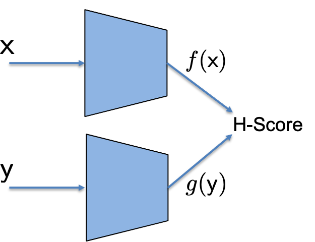
Now we can imagine a neural network as shown in the figure, where we use two forward neural networks with inputs $\mathsf x$ and $\mathsf y$ separately, each can have its own network architecture of choice, to generate $k$-dimensional features $\underline{f}(\mathsf x)$ and $\underline{g}(\mathsf y)$. Together the two set of features are put together to evaluate the H-score, and we can back propagate the gradients to adjust the network weights to maximize the H-score. We call such a network the H-score Network.
Remarks
-
Empirical Average: In the definition, all expectations are taken with respect to $P_{\mathsf {xy}}$. If the integrand only depends on one of the random variables, then the corresponding marginal distribution $P_{\mathsf x}$ or $P_{\mathsf y}$ can be used instead. When we use a batch of samples instead of the model to compute, the expectations are replaced by the empirical averages. In such cases we compute the rank-$k$ approximation of the empirical joint distribution. There is a convergence analysis on how many samples are required to ensure a desired accuracy of the result, which is out of the scope of this page.
-
Local Approximation: The local approximation is required in the derivation of the H-score. In other words, it is required when we want to justify the maximization of the H-score as solving (approximately) the modal decomposition problem and hence picking the informative features. We will for the rest of this post and all followup posts that use the H-score adopt this approximation. One particular consequence is that we no long distinguish between the $\mathrm{PMI}$ function and the approximated version $\widetilde{\mathrm{PMI}}$.
-
Constraints: The hope is to use H-score networks to compute the rank-$k$ approximation of the PMI function and hence the modal decomposition up to $k$ modes. The main difference as we stated is that the constraints to keep the feature functions in the standard form, orthonormal and descending order of correlation, are not enforced in the H-score networks.
a. There are some “hidden force” that helps us to get feature functions in the desired form, which will be discussed in details later. At this point, one can observe that the features that maximizes the H-score must be zero mean. This is because the first term in the definition does not depend on the means $\mathbb E[\underline{f}]$ and $\mathbb E[\underline{g}]$; and the 2nd term is optimized if all features have zero-mean, $\mathbb E[\underline{f} \cdot \underline{f}^T]$ and $\mathbb E[\underline{g} \cdot \underline{g}^T]$ becomes $\mathrm {cov}[\underline{f}]$ and $\mathrm{cov}[\underline{g}]$, which is in a more “natural” form.
b. The other aspects of the feature functions are less controllable in H-score networks. We cannot make sure the feature functions are normalized or orthogonal to each other. In fact, if we think of the PMI function as a matrix over $\mathcal {X\times Y}$, and our goal is to approximate this matrix by the product of a $\vert\mathcal X\vert \times k$ matrix of $f$ features and a $k \times \vert\mathcal Y\vert$ matrix of transposed $g$ features, then it is clear that any invertible linear combinations ($k\times k$ matrix multiplied on the right) of the $f$ feature matrix can be canceled by the inverse operations on the $g$ matrix. As a result, there are infinitely many equally good optimizers of the H-score. The only guarantee one can have is that optimizing the H-score can give a set of $k$ features that span the same subspace as $f^\ast_1, \ldots, f^\ast_k$. We will address is issue in the next post.
$\blacktriangle$ Demo 1: H-score Network
Here is a colab demo of how to implement an H-score network to learn the first mode, where the learned features are compared with theoretical results.
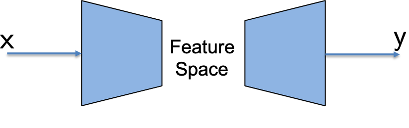
Feature Space Operations
The difference between an H-score network and the conventional neural network is illustrated in the figure. One can think the forward computing of a neural network as an “encoding” process to extract features from the input $\mathsf x$, followed by a “decoding” process to use the feature values to predict the value of the label $\mathsf y$. What an H-score network does is to turn the decoder around, and use a loss metric for features, the H-score, to both the features of $\mathsf x$ and the features of $\mathsf y$.
 |
 |
| Conventional Neural Network |
H-Score Network |
Conceptually, this is a pleasant change as we now have direct access to both sides of feature functions. The following is a quick example where our dataset consists of unordered $\mathsf{(x,y)}$ pairs, in which case we know the feature functions on $\mathsf x$ and $\mathsf y$ must be the same. In H-score networks we can tie the two networks to train them together. In other cases H-score networks often make it easier to incorporate known structural constraints in the extraction of feature functions.
In the literature, the focus on “feature space representation” or “semantics space” is a popular concept in many fields, such as in recommendation systems, in word2vec (or other xxx2vec), etc. This H-score based method has the following advantages:
-
Since the loss metric H-score is defined on the feature space, our feature extraction process does not require the correct prediction of label values based on the extracted features. This is particularly important when we only want to extract a very small number of features, which by itself cannot carry sufficient information for meaningful predictions, but can still be useful in a larger system such as distributed decision making.
-
As we define the H-score from a low rank approximation, there is a clear connection to the modal decomposition problem, which under local approximations is related to concepts in correspondence analysis and information theory. Thus the extracted features with this method often come with a clear optimality statement and are easier to interpret.
-
The local approximation put the feature functions in a Hilbert space, within which more complex operations such as projections can be carried out, which is the topic of the next post, and soon shown to be critical for multi-variate problems.
H-score Network, Conventional Neural Network, and SVD
In addition to H-score network, we have also seen two quite different approaches to computing modal decomposition and extracting features: one is to train a conventional classification network to predict $\sf y$ from $\sf x$, as we did in the demo of previous page; the other is to directly compute the SVD from the joint distribution matrix, as we did in the “oracle” class of previous demos.
Then it comes to the question on what essentially distinguishes H-score networks from these two. The short answer from an implementation perspective would be: the other two approaches cannot work if the data $\sf y$ has a rather large cardinality (or is even continuous). Specifically, the computation of SVD requires dealing with an $\vert \mathcal{X}\vert $ by $\vert \mathcal{Y}\vert $ frequency table, and the classification network requires a weight matrix of $\vert \mathcal{Y}\vert $ columns in the last layer. For high-dimensional $\sf y$, such as image/audio/text, it is impossible to estimate, process, or even store such a frequency table or weight matrix since the cardinality $\vert \mathcal{Y}\vert $ is too large.
From an information perspective, there is an essential difference between a categorical $\sf y$ and general $\sf y$. If $\sf y$ is categorical, for given two entries in $\mathcal{Y}$, we only distinguish whether they are identical or not. But for general $\sf y$, e.g., image/text, we can also talk about which two observations are closer. However, the above two approaches simply ignore the information of such closeness.
$\blacktriangle$ Demo 2: H-score for Sequential Data
Here is a colab demo to demonstrate how we apply H-score network to learn the dependence structure among high-dimensional data. Again, we generate the dataset from given probability laws to help us analyze the trained results and compare them with theoretical optimal values. However, unlike previous demos where $\sf x$ and $\sf y$ are categorical, here $\sf x$ and $\sf y$ are both sequences, and the cardinalities $\vert\mathcal{X}\vert$, $\vert\mathcal{Y}\vert$ are way larger than the sample size.
Going Forward
H-score networks is our first step in processing based on modal decomposition. It offers some moderate benefits and convenience in the standard bi-variate “data-label” problems. To us, it is more of a conceptual step, where our focus of designing neural networks is no longer to predict the labels, but rather shifted to designing the feature functions, since our loss metric is now about the features functions. In a way this is better aligned with our goals, since these features are indeed the carrier of our knowledge, and we would often need to store, exchange, and even use these features for multiple purposes, in the more complex multi-variate problems.
In our next step, we will develop one more tool to directly process the feature functions, which is in a sense to make projections in the functional space, using neural networks. This will be a useful addition to our toolbox before we start to address multi-variate learning problems.