The Key Points
In our previous posts, we developed a geometric view of the feature extraction problem. We started with the geometry of functional spaces by defining inner products and distances, and then relating the task of finding information carrying features to these geometric quantities. Based on this approach, we proposed the H-Score networks as one method to learn the informative feature functions from data using neural networks. Here, we describe a new architecture, the nested H-Score network, which is used to make projections in the functional space with neural networks. Projections are perhaps the most fundamental geometric operations, which are now made possible, and efficient, through the training of neural networks. We will show by some examples how to use this method to regulate the feature functions, incorporate external knowledge, prioritize or separate information sources, which are the critical step towards multi-variate and distributed learning problems.
 |
| H-Score Network |
Previously
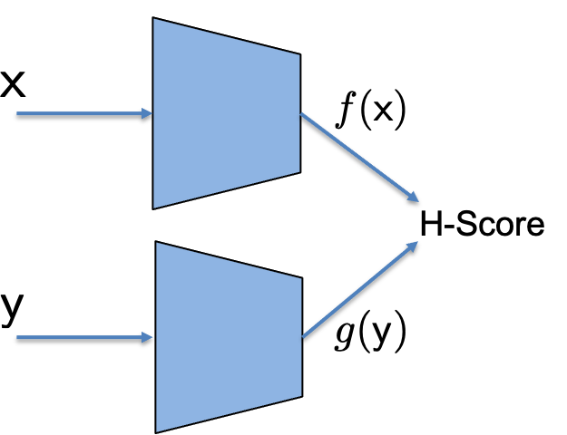
In this page, we defined H-Score network as shown in the figure, where the two sub-networks are used to generate features of $\mathsf x$ and $\mathsf y$: $\underline{f}(\mathsf x), \underline{g}(\mathsf y)\in \mathbb R^k$. The two features are used together to evaluate a metric, the H-score,
\[H(\underline{f}, \underline{g}) =\mathrm{trace} (\mathrm{cov} (\underline{f}, \underline{g})) - \frac{1}{2} \mathrm{trace}(\mathbb E[\underline{f} \cdot \underline{f}^T] \cdot \mathbb E[\underline{g} \cdot \underline{g}^T])\]
where the covariance and the expectation are evaluated by the empirical averages over the batch of samples. We use back-propagation to train the two networks to find
\[\underline{f}^\ast, \underline{g}^\ast = \arg\max_{\underline{f}, \underline{g}} \; H(\underline{f}, \underline{g}).\]
The resulting optimal choice $\underline{f}^\ast, \underline{g}^\ast$ are promised to be a good set of feature functions. They are the solutions of the approximated and unconstrained version of the modal decomposition problem, which has connection to a number of theoretical problems, and, in a short sentence, picks “informative” features.
The H-Score network is an approximation of modal decomposition because of the imperfect convergence and the limited expressive power of the neural networks, the randomness in the empirical averages due to the finite batch of samples, and the local approximation we used when formulating the modal decomposition. For the rest of this page, we will take the local approximation for granted. For example, we will not distinguish between the function
\(\mathrm{PMI}_{\mathsf {xy}} = \log \frac{P_{\mathsf {xy}}}{P_\mathsf x\cdot P_\mathsf y} \; \in \; \mathcal {F_{X\times Y}}\)
and its approximation
\(\widetilde{\mathrm{PMI}}_{\mathsf {xy}} = \frac{P_{\mathsf {xy}} - P_{\mathsf x}\cdot P_{\mathsf y}}{P_\mathsf x\cdot P_{\mathsf y}} \; \in \; \mathcal {F_{X\times Y}}\)
The Constraints
In practice, it is more problematic that the H-Score network, as well as other neural network based approaches, generates unconstrained features. In the definition of modal decomposition, the ideal modes $(\underline{f}^\ast, \underline{g}^\ast) = {(f^\ast_i, g^\ast_i), i=1, \ldots k }$ satisfy:
- normalized: $\mathrm{var}[f_i^\ast (\mathsf x)] = \mathrm{var}[g_i^\ast(\mathsf y)] = 1, \; i=1, \ldots, k$;
- orthogonal: $\mathbb E[f_i^\ast(\mathsf x)f_j^\ast(\mathsf x)] = \mathbb E[g_i^\ast(\mathsf y)g_j^\ast(\mathsf y)] =0 , \; \forall i \neq j$
- in descending order: $\sigma_i = \mathbb E[f^\ast_i(\mathsf x)g^\ast_i(\mathsf y)]$ non-increasing as $i$ increases.
These regulations are all desirable properties in practice. Unfortunately, the H-score network generates features that in general without these constraints. This can be easily seen from the definition: for any invertible matrix $A \in \mathbb R^{k\times k}$,
\[H(\underline{f}, \underline{g}) = H(A\underline{f}, A^{-1} \underline{g})\]
That is, any linear combination of the $k$ feature functions in $\underline{f}$ can be cancelled by a corresponding inverse linear transform on $\underline{g}$, which result in an equivalent solution. Thus H-score cannot distinguish between such solutions. As a result, the best thing we can hope is to get a collection of feature functions that span the same subspace as the optimal choices for the modal decomposition problem.
The idea of viewing the subspace spanned by a collection of features as the carrier of information is itself worth some discussions. In this page, however, we will focus on how to modify the H-Score network to enforce some of these constraints. It turns out that the key is to have a new operation to make projections of feature functions.
Nested H-Score Network
We start by consider the following problem to extract a single mode from a given model $P_{\mathsf {xy}}$, but with a simple constraint: for a given function $\bar{f} : \mathcal X \to \mathbb R$, we would like to find a mode, i.e. a pair of features $f(\cdot), g(\cdot)$, as the optimal rank-$1$ approximation as before, but under the constraint that $f \perp \bar{f}$, i.e. $\mathbb E_{\mathsf x \sim P_\mathsf x}[f(\mathsf x) \cdot \bar{f}(\mathsf x)] = 0$:
\[(f^\ast, g^\ast) = \arg\min_{\small{\begin{array}{l}(f, g): f\in \mathcal {F_X}, g \in \mathcal {F_Y}, \\ \qquad \quad \mathbb E[f(\mathsf x)\cdot \bar{f}(\mathsf x)]=0\end{array}}} \; \left\Vert \mathrm{PMI} - f \otimes g \right\Vert^2\]
where $\mathrm{PMI}$ is the pointwise mutual information function with $\mathrm{PMI} (x,y) = \log \frac{P_{\mathsf {xy}}(x,y)}{ P_\mathsf x(x)P_\mathsf y(y)}$, for $x\in \mathcal X, y \in \mathcal Y$.
 |
| Nested H-Score Network to find features orthogonal to a given $\bar{f}$ |
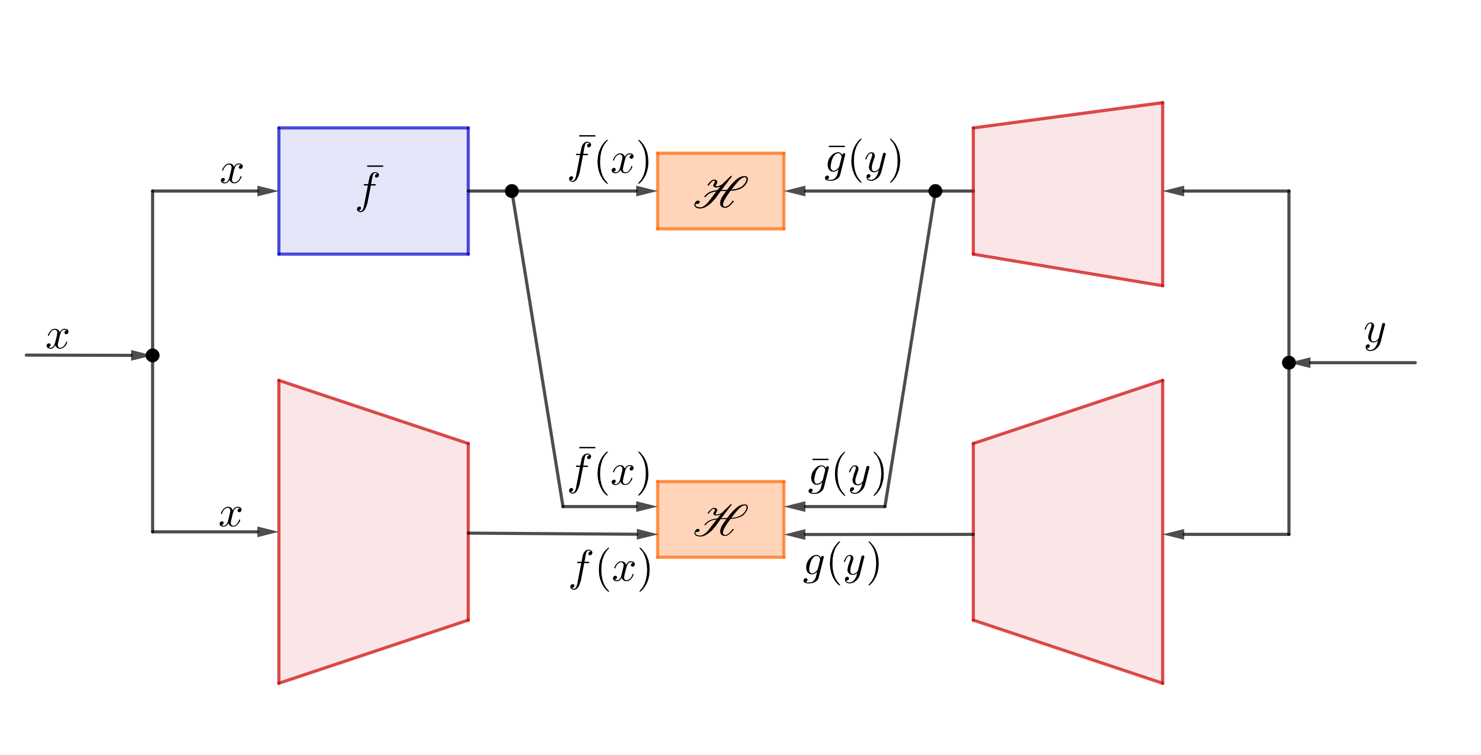
While there are many different ways to solve optimization problems with constraints, the figure shows the nested H-Score network we use, which is based on simultaneously training a few connected neural networks.
In the figure, the blue box $\bar{f}$ is assumed to be the given function. The three red sub-networks are used to generate $1$-dimensional feature functions $\bar{g}, f$ and $g$. (As we will see soon, that $f$ and $g$ can in fact be higher dimensional, hence drawn slightly bigger in the figure.)
With a batch of samples $(x_i, y_i), i=1, \ldots, n$, the network is trained with the following procedure.
Training for Nested H-Score Networks
-
Each sample pair $(x_i, y_i)$ is used to compute $\bar{f}(x_i)$, and forward pass through the neural networks to evaluate $f(x_i), \bar{g}(y_i), g(y_i)$;
-
The output $\bar{f}(\mathsf x_i), \bar{g}(\mathsf y_i), i=1, \ldots, n$ are used together to evaluate the H-score for $1$-D feature pairs shown on the top box; the two pairs of features $[\bar{f}, f]$ and $[\bar{g}, g]$ are used to evaluate a 2-D H-score in the lower box. In both cases the expectations are replaced by the empirical means over the batch;
-
The gradients to maximize both the H-scores are back propagated through the networks to update weights. In particular, the sum of the gradients from the two H-scores are used to train $\bar{g}$; only the gradients from the bottom H-score are used to train $f$ and $g$ networks.
-
Iterate the above procedure until convergence.
To see how this achieves the goal it might be easier to look at a slightly different way to train the network, namely the sequential training. Here, we first only use the top H-Score to train the feature function $\bar{g}$ only. From the definition of the H-Score, we know this finds $\bar{g}^\ast$ by solving the following optimization.
\[\begin{align}
\bar{g}^\ast = \arg \min_{\bar{g}} \; \left\Vert\mathrm{PMI} - \bar{f} \otimes \bar{g}\right\Vert^2
\end{align}\]
After that, we freeze $\bar{g}^\ast$, and use the bottom H-Score to train both $f$ and $g$. With this choice of $\bar{g}^\ast$, we have that the minimum error, $\mathrm{PMI} - \bar{f} \otimes \bar{g}^\ast$ must be orthogonal to $\bar{f}$ in the sense that for every $y$, $\mathrm{PMI}(\cdot, y)$ as a function over $\mathcal X$ is orthogonal to $\bar{f}$, since otherwise the L2 error can be further reduced. The maximization of the bottom H-Score is now the following optimzation problem:
\[\begin{align}
(f^\ast, g^\ast) = \arg\min_{f, g} \; \left\Vert \mathrm{PMI} - (\bar{f}\otimes \bar{g}^\ast + f\otimes g) \right\Vert^2
\end{align}\]
This can be read as the rank-$1$ approximation to $(\mathrm{PMI}- \bar{f}\otimes \bar{g}^\ast)$, which is orthogonal to $\bar{f}$. So the resulting the optimal choice of $f^\ast$ must also be orthogonal to $\bar{f}$ as we hoped.
A few remarks are in order now.
-
One should check that at this point if we freeze the choicec $f^\ast, g^\ast$ and allow $\bar{g}$ to update, $\bar{g}^\ast$ defined in (1) actually maximizes both H-Scores. Thus if we turn the sequential training into iteratively optimize $\bar{g}$ and $f, g$, we get the same results.
-
In practice, we would not wait for the convergence of one step before starting the next, and thus the proposed training procedure is what we call
simultaneous training, where all neural networks are updated simultaneously. It can be shown that in this setup the results are the same as those from the sequential training. However, in our later examples of using the nested H-Score architectures, often with subtle variations, we need to discuss in each case whether this still holds.
-
There are of course other ways to make sure the learned feature function to be orthogonal to the given $\bar{f}$. For example one could directly project the learned feature function against $\bar{f}$. Here, the projection operation is separated from the training of the neural network, rasing the issue that the objective function used in training may not be perfectly aligned with that in the space after the projection. In nested H-Score networks, the orthogonality constraint is naturally included in the training of the neural networks. There is also some additional flexibility with this design. For example in several followup cases using nested H-Score we would learn $\bar{f}$ from data at the same time.
Example: Ordered Modal Decomposition
We now go back to the problem that we started this page with: we would like to use the nested H-Score network to compute the modal decomposition, but wish the resulting modes to be in the standard form. That is, we want the extracted feature functions to be orthonormal, and the modes to be in a descending order of strengths.
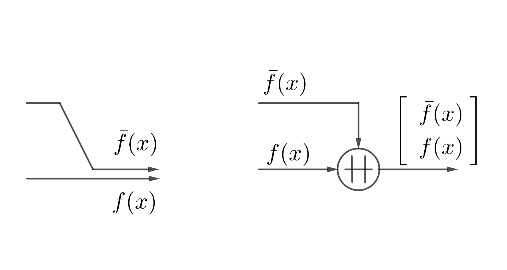
As we will use the nested structure repeatedly, to avoid having too many lines in our figures, we will adopt a new concatenation symbol, “$\,+\hspace{-.7em}+\,$”, where simply takes all the inputs to form a vector output. In some drawings such an operation to merge data is simply denoted by a dot in the graph, but here we use the special symbol to emphasize the change of dimensionality. For example, the concatenation operation in the nest H-Score network is replaced with a new figure as follows.
 |
| The Concatenation Symbol |
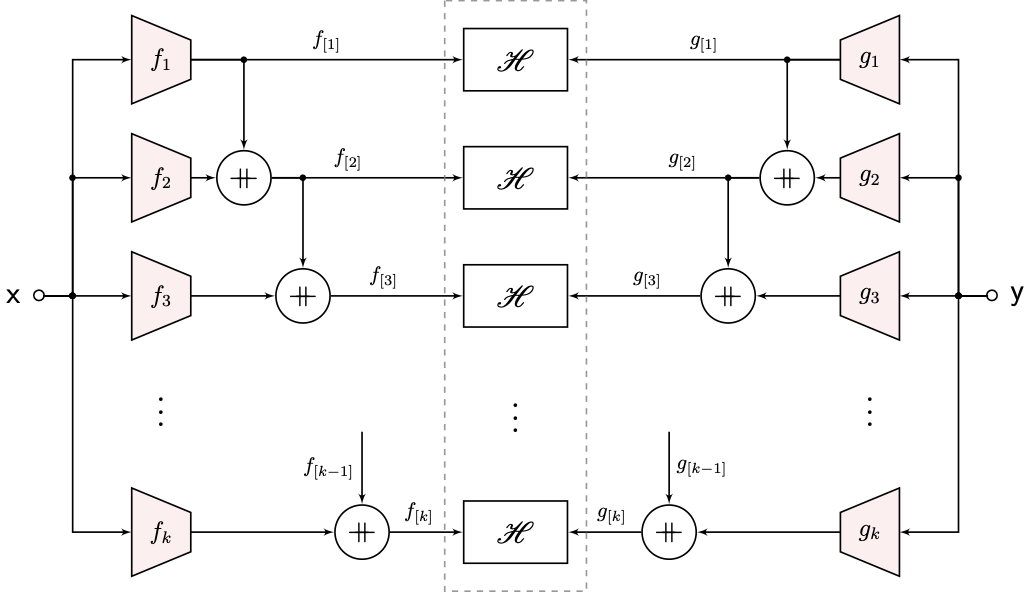
Now the nested H-Score network that would generate orthogonal modes in descending order is as follows.
 |
| Nested H-Score Network for Ordered Modal Decomposition |
In the figure, we used the notation $f_{[k]} = [f_1, \ldots, f_k]$. Again, it is easier to understand the operation from sequential training. We can first train the $f_1, g_1$ block with the top H-Score box, and this finds the first mode $f^\ast_1, g^\ast_1 = \zeta_1(P_{\mathsf {xy}})$. After that, we train $f_2, g_2$ with the first mode freezed. The nested network ensures that the resulting mode to be orthogonal to the first mode, which by definition is the second mode $\zeta_2(P_{\mathsf {xy}})$. Following this sequence we can get the $k^{th}$ mode that is orthogonal to all the previous $k-1$ ones. It takes a proof to state that we can indeed simultaneously train all sub-networks, which we omit from this page.
$\blacktriangle$ Pytorch Implementations
The first colab demo illustrates how to implement a nested H-score network in pytorch, where we compare the extracted modes with the theoretical results.
As in the previous post, we can also apply the nested H-score on sequential data. In the second demo, we compare the nested H-score with the vanilla H-score, which also demonstrates the impact of feature demensions.
Going Forward
Nested H-Score Networks is our way to make projections in the space of feature functions, using interconnected neural networks. This is a fundamental operation in the functional space. In fact, in many learning problems, especially when the problem is more complex, such as with multi-modal data, multiple tasks, distributed learning constraints, time-varying models, privacy/security/fairness requirements, or when there is external knowledge that needs to be incorporated in the learning, such projection operations become critical. In our next post, we will give one of such examples with a multi-terminal learning problem.